目次
TensorFlow (version 1.4), TensorFlow Probability, Edwards2 の勉強のために、最尤推定とベイズ推定の各種解法で、潜在変数ありの場合に代表的な混合ガウスモデルを解く。潜在変数なしの線形回帰はこちら。
Jupyter Notebook はここ。Plotly まわりのために BITS という自作パッケージを使っているので、コードを動かす場合はインストールする。
Tensorflow 関連のインポートは以下の通り。今回は Eager Execution を使用する。
import tensorflow as tf
import tensorflow_probability as tfp
from tensorflow_probability import edward2 as ed
tfd = tfp.distributions
tfb = tfp.bijectors
tf.enable_eager_execution()
モデル
上のガウス分布 個の混合分布から 個のデータ を観測したとする。データ が属する分布を で表し、 は混合ガウス分布
に従うとする。ただし、 で は 2 次元単位行列。ここでは分布ごとに分散は異なるが、同じ分布の各次元では分散は同じとしている。
データ生成
定数は以下の通り。
D = 2   # number of dimensions of data
K = 3   # number of mixture components
N = 1000 # number of data (= observations)各パラメタは適当な一様分布から決めた。pi_trueは真の混合比率。
dtype = np.float32
mu_true = np.random.uniform(-1, 1, [D, 2]).astype(dtype)
sigma_true = np.random.uniform(0.05, 0.1, [D, 1]).astype(dtype)
z_true = np.random.choice(2, N)
pi_true = np.expand_dims(np.unique(z_true, return_counts=True)[1] / N, axis=1).astype(dtype)
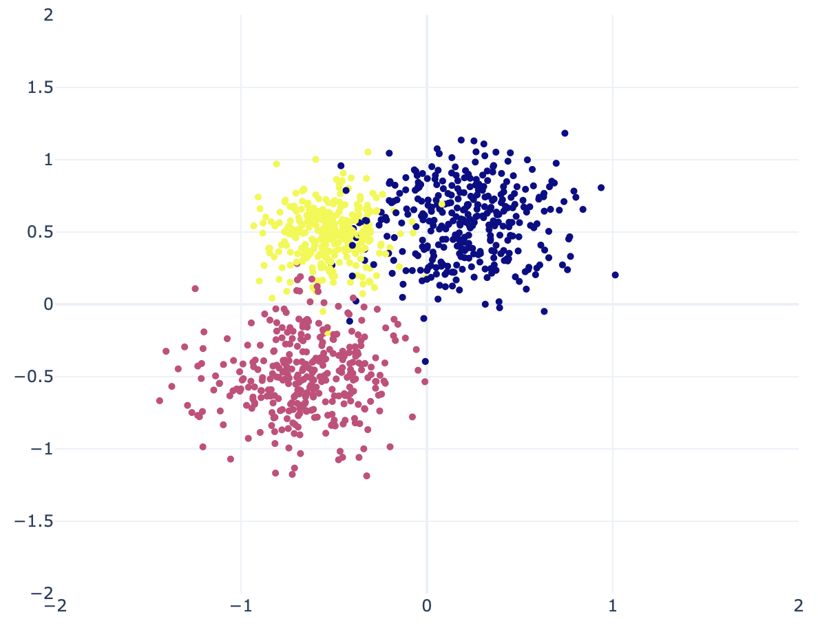
x = np.array([np.random.multivariate_normal(mu_true[z_true[i]], sigma_true[z_true[i]] * np.identity(D)) for i in range(N)]).astype(dtype)生成したデータを 2 次元平面にプロットすると以下の通り。分布が気に入らなければ再度上のコードを実行して生成し直す。
最尤推定
共分散行列がすべて の混合ガウス分布の対数尤度最大化
は、k-means クラスタリングの目的関数最小化
と同じ。
EM アルゴリズム (k-means クラスタリング)
sklearnがあるのにフルスクラッチで実装するのはさすがに面倒だったので手抜き。一応 Tensorflow にも tf.contrib.factorization.KMeans というものはあるらしい。バージョン 2 で残るかは分からない。
from sklearn.cluster import KMeans
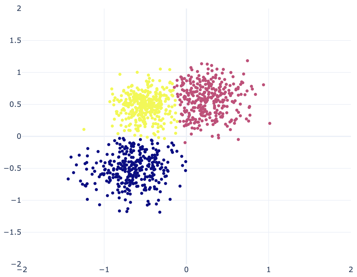
kmeans = KMeans(n_clusters=K, random_state=0).fit(x)結果は以下の通り。k-means は等分散を仮定しているため、分布ごとに分散が大きく異なる場合はうまくいかない。
EM アルゴリズム (分散も推定)
TODO
ベイズ推定
生成モデルは以下のようにする。
ただし、 は分布の混合比率で、 はハイパーパラメタ。事後分布の形は以下の通り。
ギブスサンプリング
TODO
ハミルトニアンモンテカルロ法
ハイパーパラメタは以下のようにした。データ生成の際のパラメタとあまりかけ離れた設定にならないようにする。
alpha0 = np.ones(K, dtype=dtype) / K
mu0 = np.zeros([K, D], dtype=dtype)
s0 = np.ones([K, D], dtype=dtype)
a0 = np.full(K, 10, dtype=dtype)
b0 = 0.5同時分布を計算する関数log_jointおよびそれを使って非正規化事後確率を計算する関数unnormalized_posteriorを定義する。 を消去するためにtfd.MixtureSameFamilyを使う。 個のガウス分布はまとめてtfd.Independentで扱う。このとき、tfd.Independent(tfd.Normal(loc, scale))のlocとscaleのshapeはともに(K, D)である必要がある。今回は 1 つのガウス分布の各次元の分散は同じとしているので少しややこしい。
rv_pi = tfd.Dirichlet(alpha0, name="pi")
rv_mu = tfd.Independent(tfd.Normal(mu0, s0), name="mu")
rv_var = tfd.InverseGamma(a0, b0, name="var")

def tf_repeat(a, multiples, axis):
    """np.repeat() in tf."""
    return tf.concat([a for i in range(multiples)], axis=axis)

def log_joint(pi, mu, var, x):
    rv_x = tfd.MixtureSameFamily(tfd.Categorical(probs=pi),
                                 tfd.Independent(tfd.Normal(mu, tf_repeat(tf.sqrt(var)[:, tf.newaxis], D, axis=1))))
    sum_log_prob = tf.reduce_sum(tf.concat([rv_x.log_prob(x),
                                            rv_pi.log_prob(pi)[..., tf.newaxis],
                                            rv_mu.log_prob(mu),
                                            rv_var.log_prob(var)], axis=-1))
    assert not np.isnan(sum_log_prob), f"Nan, pi={pi}, mu={mu}"
    return sum_log_prob

def unnormalized_posterior(pi, mu, var):
    return log_joint(pi=pi, mu=mu, var=var, x=x_observed)
あとは推移核を作る。ハミルトニアンモンテカルロ法ではパラメタに対する制約をサンプリング中に取り入れることはできないため、 は MCMC 中成り立たない。そこで、tfb.SoftmaxCenteredを使って一旦 を制約無しの空間上の変数に変換し、MCMC が終わった後に元の制約のある変数へと引き戻す (これは自動でやってくれる)。Bijector を使う場合はtfp.mcmc.HamiltonianMonteCarloをtfp.mcmc.TransformedTransitionKernelでラップする必要がある。
step_sizeとn_leapfrog_stepsの値は下の MCMC を何度か試しに回して受容率がおかしくならないように手で調整した後のもの。
step_size = 0.002
n_leapfrog_steps = 5
hmc_kernel = tfp.mcmc.TransformedTransitionKernel(
    inner_kernel=tfp.mcmc.HamiltonianMonteCarlo(unnormalized_posterior, step_size, n_leapfrog_steps),
    bijector=[tfb.SoftmaxCentered(), tfb.Identity(), tfb.Identity()])
そして、パラメタの初期値を決めて MCMC を回す。今回は各ガウス分布の平均 の初期値をすべて 0 で与えたのだが、生成したデータの分布同士の重なりが大きいためか、適当なstep_sizeとn_leapfrog_stepsではかなりの確率で のうち 1 つが途中で 0 になりlog_jointが NaN になってしまったり、受容率が 0 になってしまったりした。ちなみに公式 Jupyter Notebook では真の平均を初期値にしている (いいのか?)。そのようにした場合は、収束が早くなるためか比較的適当なステップサイズ等で大丈夫だった。
n_burnin = 1000
n_iters = 3000
pi_init = np.ones(K, dtype=dtype) / K
mu_init = np.zeros([K, D], dtype=dtype)
var_init = np.full(K, 0.05, dtype=dtype)

(pi_samples, mu_samples, var_samples), kernel_results = tfp.mcmc.sample_chain(n_iters,
                                                                              [pi_init, mu_init, var_init],
                                                                              num_burnin_steps=n_burnin,
kernel=hmc_kernel)状態遷移の受容率はnp.mean(kernel_results.inner_results.is_accepted)で分かる。今回は約 92%だった。
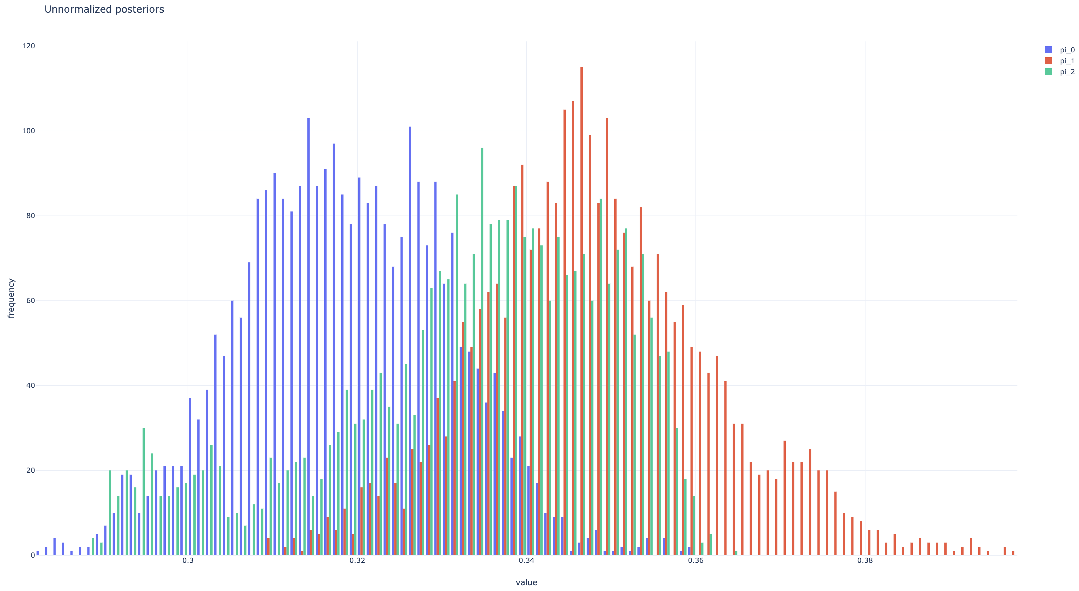
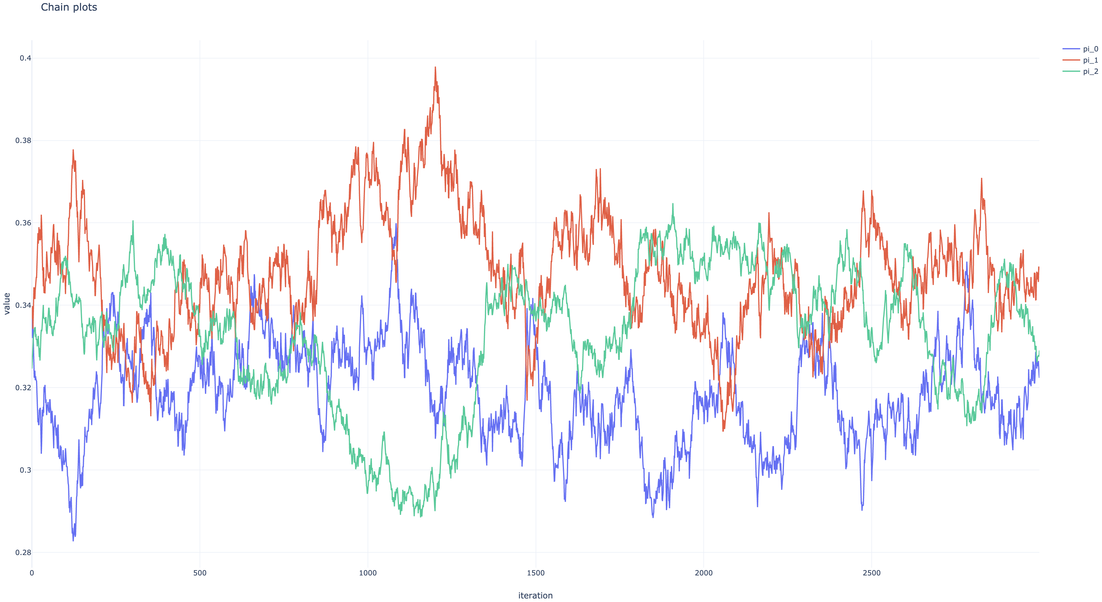
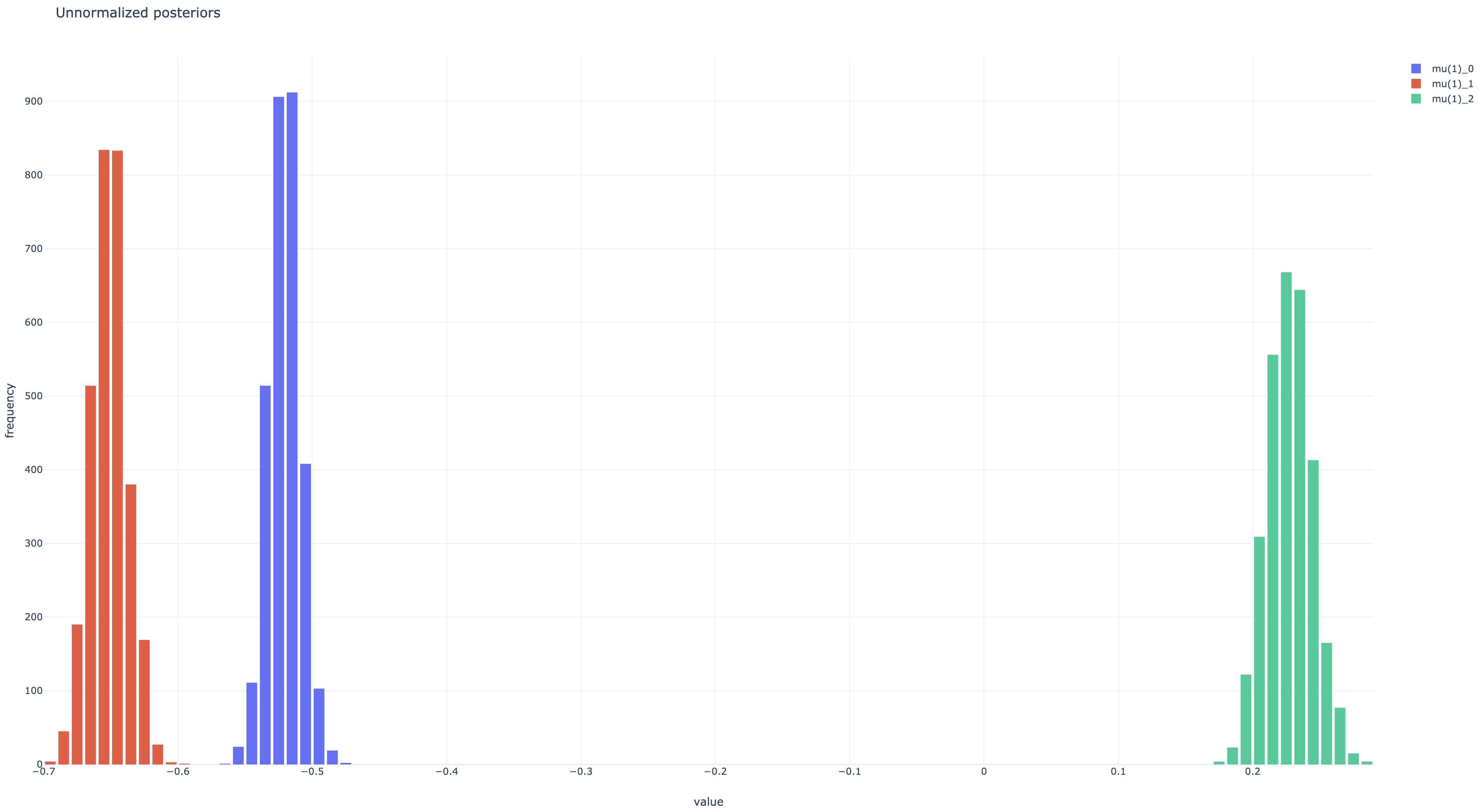
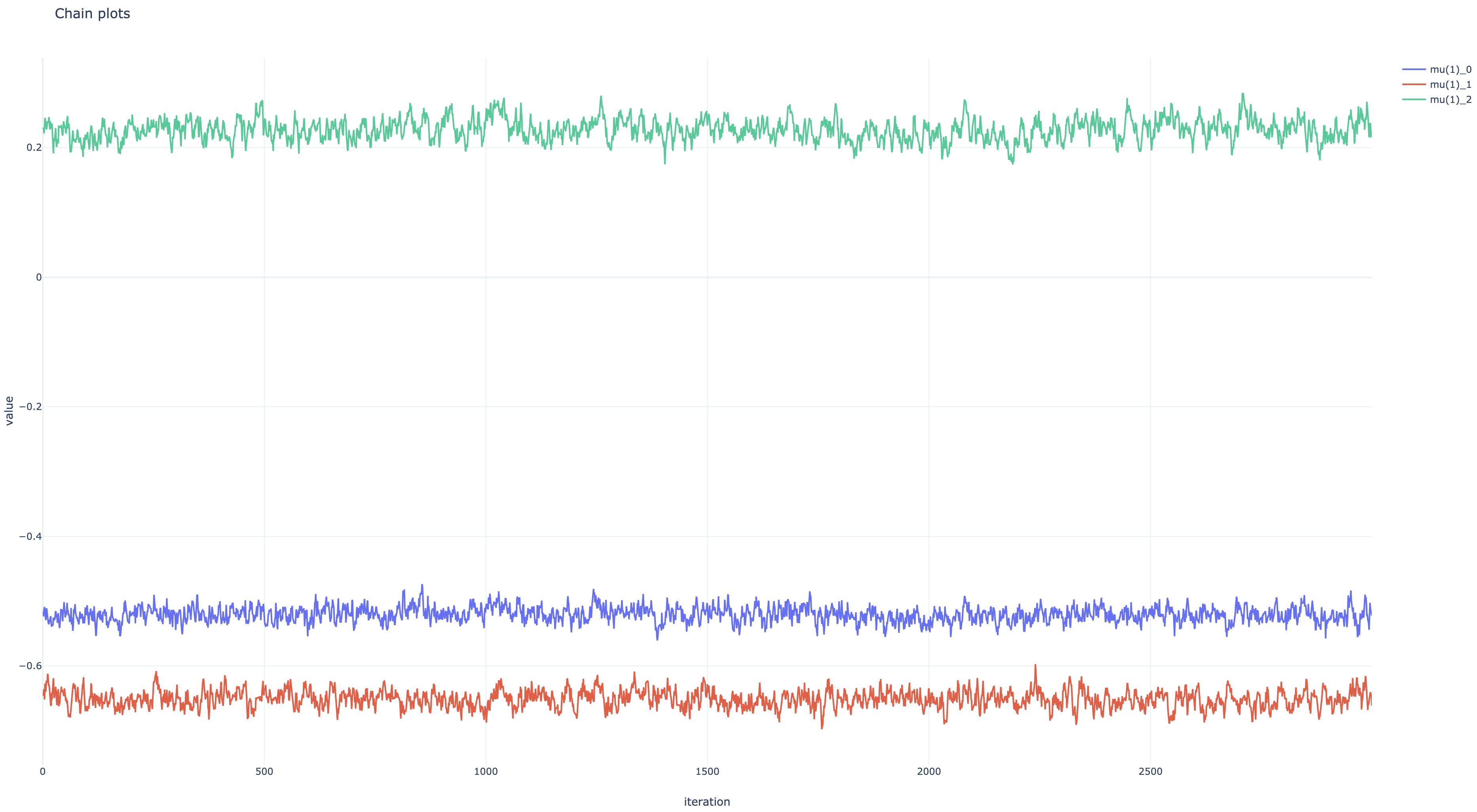
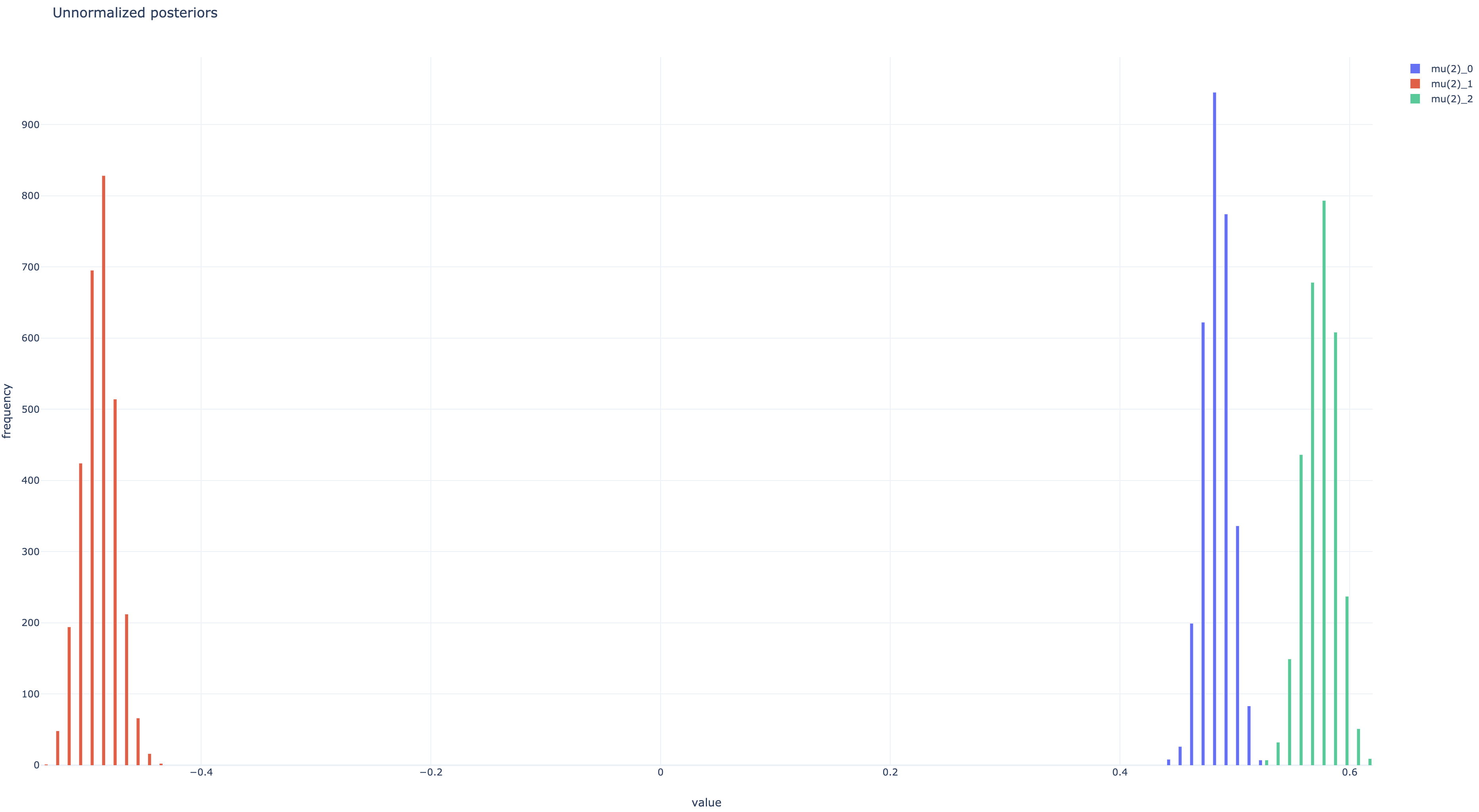
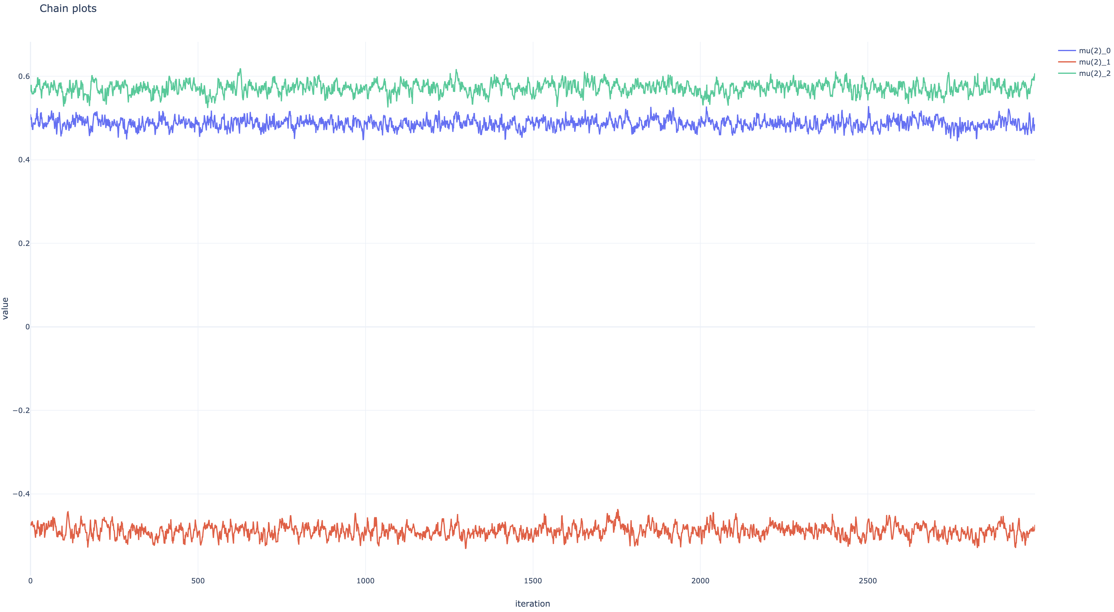
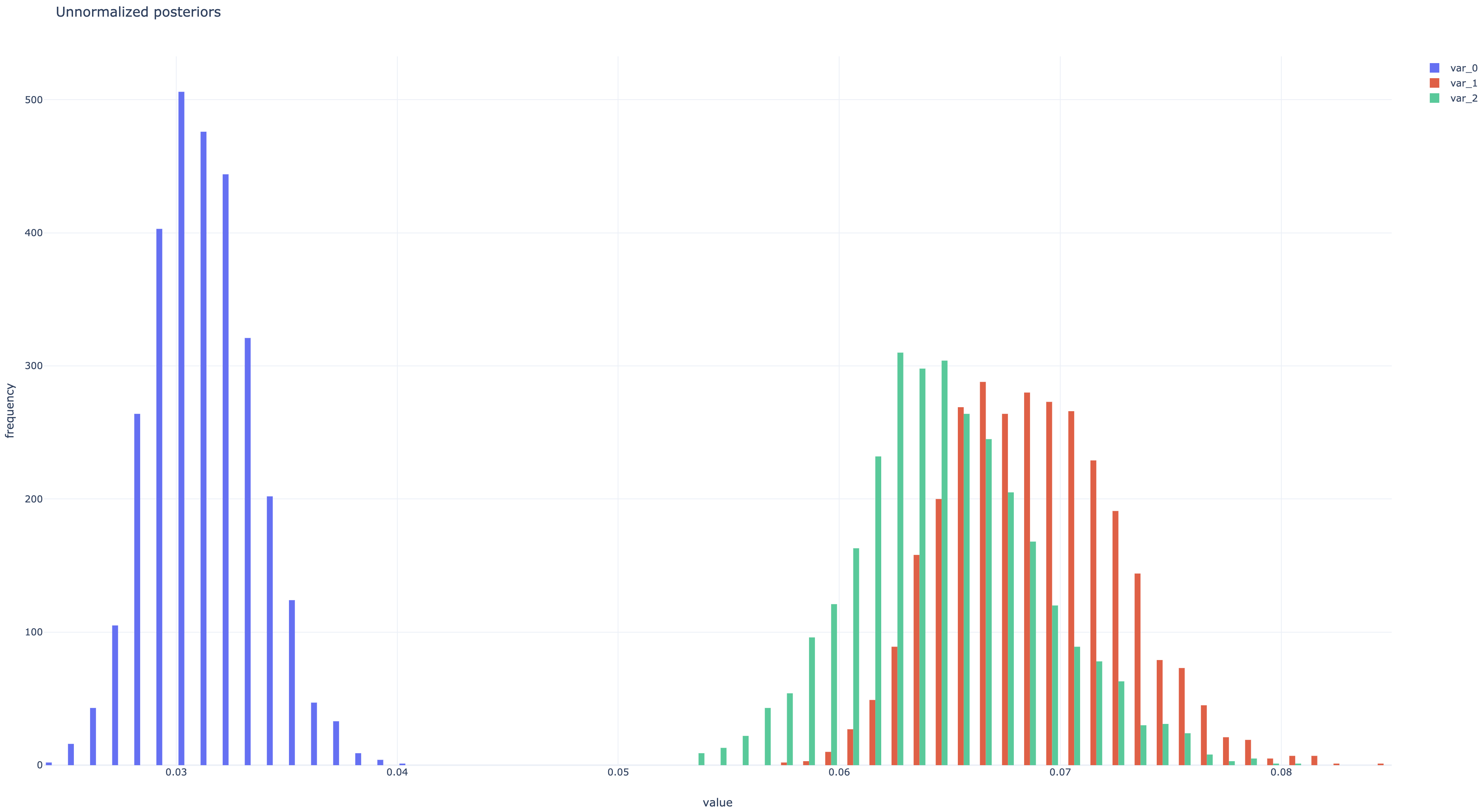
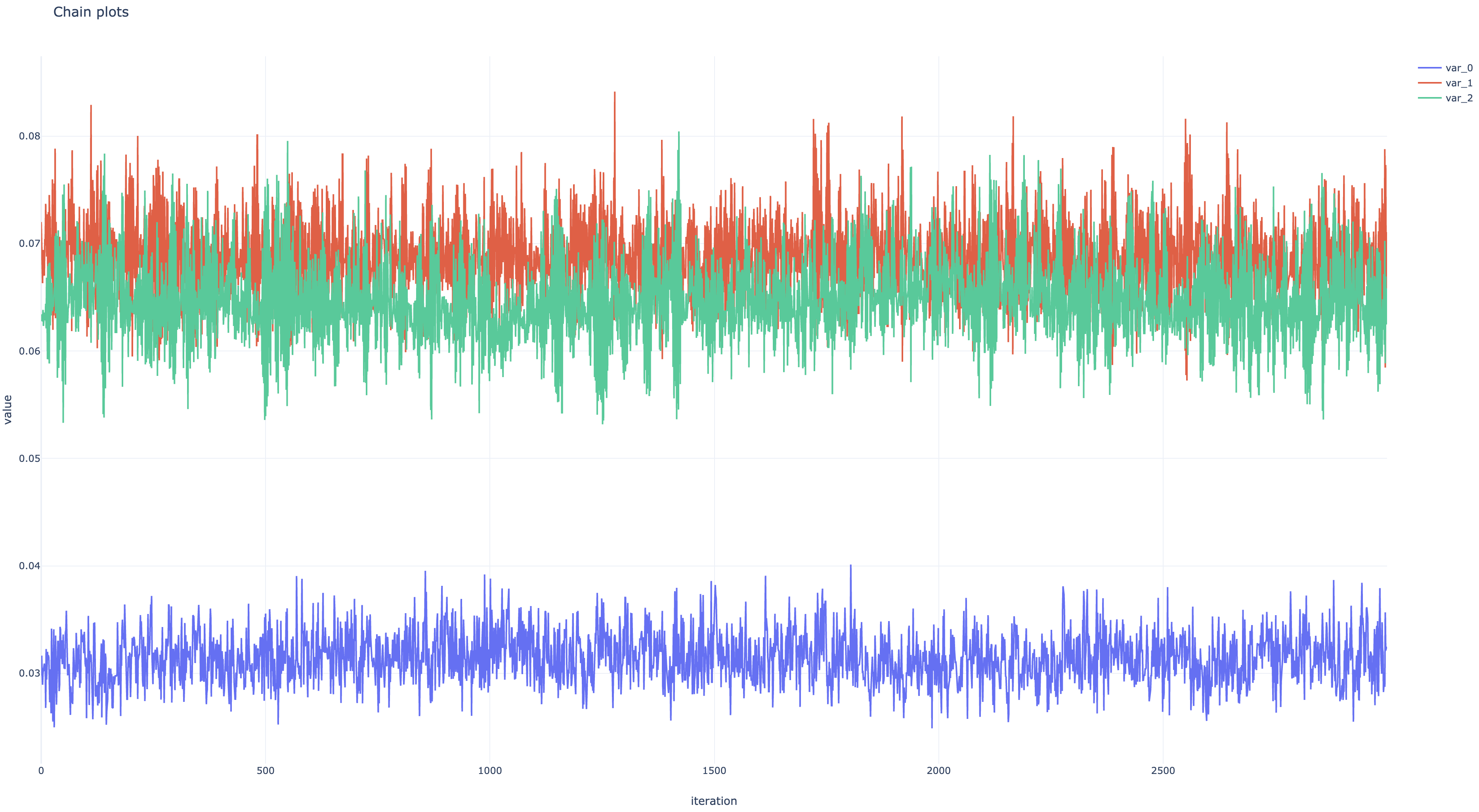
非正規化事後分布とパラメタ遷移のプロットは以下のようになった。 ともにちゃんと収束している。
変分推論
TODO